Detect Every Thing with Few Examples
使用vision-only的DINOv2作为backbone从少量图像样本中学习新类别
Motivation
开放词汇表对象检测通过用其类别名称的language embedding来表示每个类而取得了显著的成功,但作者认为使用语言作为类别的表示存在局限性:
- 某些对象很难仅用语言准确描述,或缺乏简洁的名称
- 视觉概念和语言之间的联系是不断发展的,而不是静止的,而Open Vocabulary模型只能链接在语料库中先前连接的对象和名称
- 当图像注释可用时,基于语言的分类不会利用图像注释
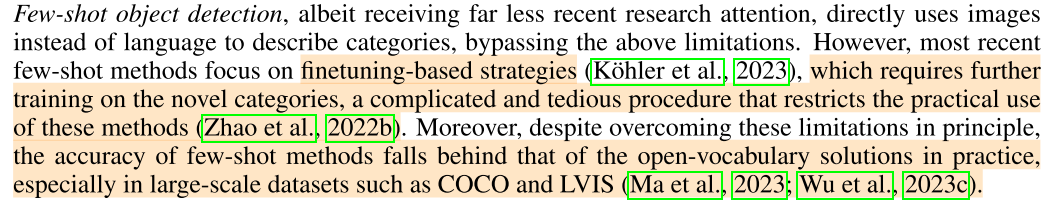
Few-shot object detection,部分方法需要在新类别上微调,限制了应用,且few-shot方法的效果不如open-vocabulary效果
作者对于open-set,open-vocabulary,few-shot的概念理解

Methodology
- New classes can be added with a few example images in an ad-hoc manner without any finetuning
- The DINOv2 backbones are kept frozen and only our detection-related layers are trained
Major Challenge:
a network trained with base classes would inevitably fixate on patterns that are only present among a few base classes, which does not align with the objective of detecting arbitrary classes
learn not only backbone features, but also maps of similarities between the features and a set of prototypes
Classification with an Unknown Number of Classes
对于不确定的类别数量:
- FSOD中的常见策略是将最后一层全连接层进行微调
- OVD则是利用类别名对应的text embedding vectors替代最后一层全连接层
- 本文中则是transform the multi-classification of $C$ classes into $C$ one-vs-rest binary classification tasks
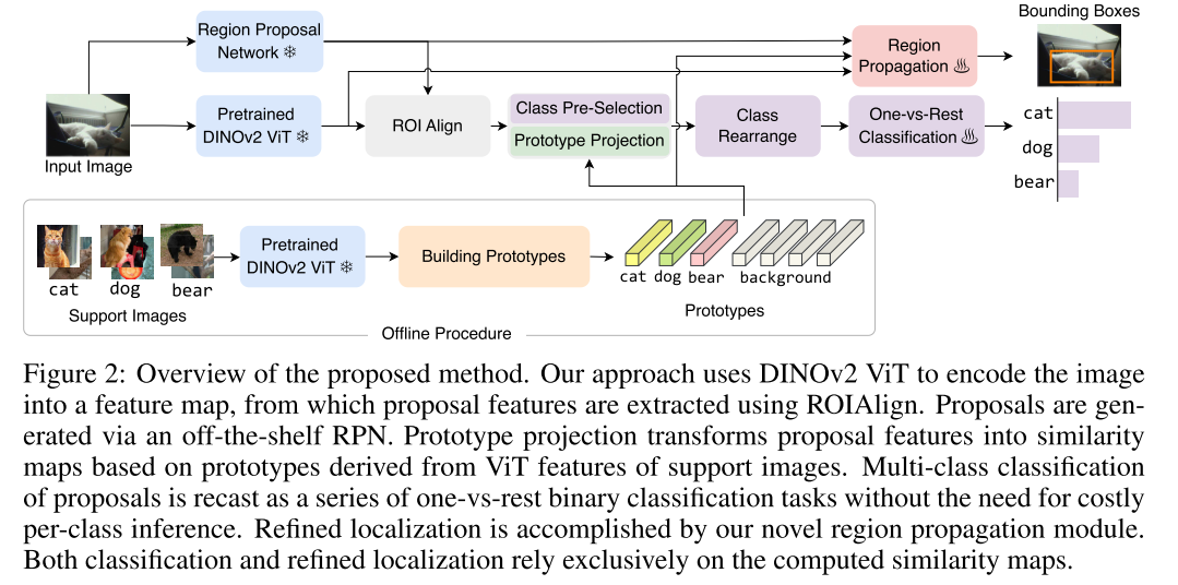
采用两阶段目标检测框架,使用离线的RPNs来生成region proposal,并从DINOv2中获取region proposal对应区域特征
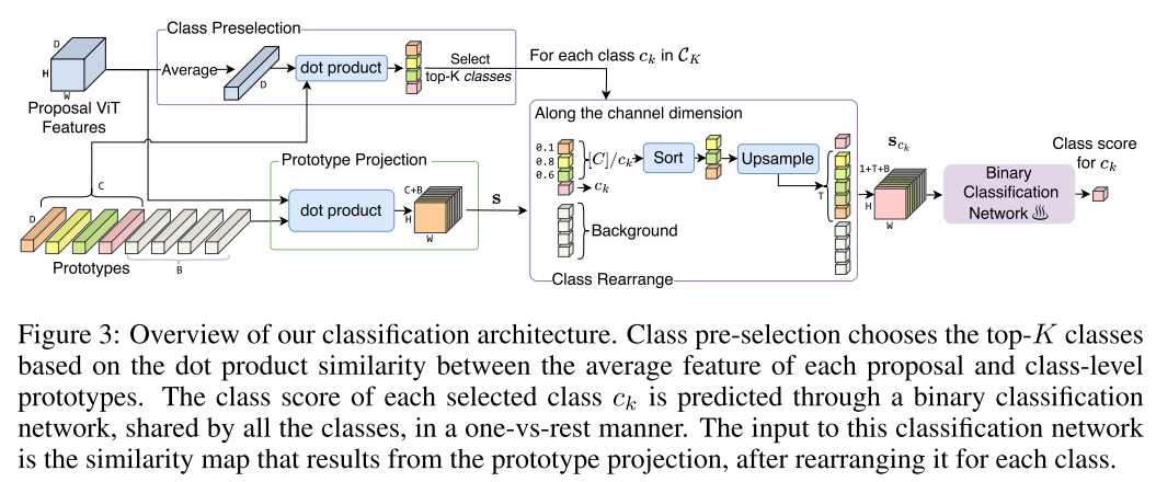
Classification architecture:
- $\overline{\mathbf{f}}=\frac{\sum_{i, j=1}^{H, W} \mathbf{f}_{i j}}{H W} \in \mathbb{R}^{D}$代表proposal的平均特征(avg pooling),用于选取top classes $\mathcal{C}_K$
- Class Preselection返回top-K个最可能的类别(使用点乘计算当前proposal平均特征和class prototypes的相似度,然后排序取top-K),用$\mathcal{C}_K$代表
Prototype projection:
- $\mathbf{f}\in\mathbb{R}^{H\times W\times D}$代表图像的特征,$D$是特征维度
- $\mathbf{p}\in \mathbb{R}^{(C+B)\times D}$代表prototypes,其中$C$代表类别数,$B$代表类别无关的背景prototypes数量
- Similarity map $s\in\mathbb{R}^{H\times W\times (C+B)}$使用下式计算:
- $\mathbf{s}_{i j c}=\sum_{d=1}^{D} \mathbf{f}_{i j d} \mathbf{p}_{c d}, \text { where }(i, j, c) \in[H] \times[W] \times[C+B]$
- 其中$[C+B]$代表$\{1,…,C+B\}$
Class Rearrange:
- 对于每一个$c_k\in C_K$,根据prototype projection中similarity map的计算方式,将Similarity map $\mathbf{s}\in\mathbb{R}^{H\times W\times (C+B)}$ rearrange为class-specific map $\mathbf{s}_{c_k}\in\mathbb{R}^{H\times W\times (1+T+B)}$
- 图中的$[C]/c_k$代表$\{1,…,c_k-1,c_k+1,…,C\}$
- $\mathbf{s}_{c_k}$的维度中,1代表类别$c_k$, $T$是$C$中除了类别$c_k$外所有类的Similarity map上采样后的维度,$B$则代表背景prototypes的数量,因此$\mathbf{s}_{c_{k}}=\operatorname{concat}\left(\mathbf{s}\left[:,:, c_{k}\right], F_{\text {rearrange }}\left(\mathbf{s}_{[C] / c_{k}}\right), \mathbf{s}[:,: C: C+B]\right)$
- $F_{\text {rearrange }}(\mathbf{x})=\left\{\begin{array}{ll}
\operatorname{upsample}(\operatorname{sort}(\mathbf{x}), T) & \text { if } T \geq C-1 \\
\operatorname{sort}(\mathbf{x})[:,:,: T] & \text { otherwise }
\end{array}\right.$ ,首先按照将$\mathbf{s}_{[C] / c_{k}}$的channel dimension对$[C]/c_k$进行排序,然后保留top $T$ classes,如果$T$超过了$C-1$则将similarity上采样到$T$。这一步将不确定的类别数量对应的不确定size特征维度$H\times W\times (C-1)$变为了固定size $H\times W\times T$ - 其中concat, upsample, sort(降序排列)都是在channel dimension进行的
- 最后class-specific similarity map $\mathbf{s}_{c_k}$被送进binary classification network并返回$c_k$类别的class score,一般取K=10(论文的主要结果都是top10,但top3已经有SoTA效果)
Our method only predicts class scores for $C_K$ and sets the others to 0. As shown in Sec. 4.2, our method surpasses SoTA even when K = 3 on both COCO (80 classes) and LVIS (1203 classes), eliminating the need for costly per-class inference.
由于只需要计算Top-K个类别, 因此避免了对每个类都进行推理
Localization with Region Propagation
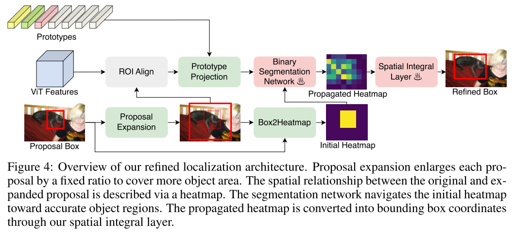
propagation procedure is implemented through binary segmentation,作者将groundtruth bboxex转换为heatmaps来训练这个分割网络
学习一个从heatmap到box相对坐标 $(c_{w}^{\text {rel }}, c_{h}^{\text {rel }},w^{\text {rel }}, h^{\text {rel }})\in [0,1]^4$的变换, 这个box相对坐标是相对expanded proposal的
Inspired by unsupervised keypoint estimation, particularly the works of IMM (Jakab et al., 2018) and Transporter (Kulkarni et al., 2019), we devise a spatial integral layer to project the propagated heatmap to box.
变换:用$\mathbf{g}\in \mathbb{R}^{H\times W}$代表logits of the propagated heatmap, 相对坐标box可以用下式来估计
$\begin{array}{l}
\left(c_{w}^{\text {rel }}, c_{h}^{\text {rel }}\right)=\sum_{i, j=1}^{H, W}\left(\frac{i}{H}, \frac{j}{W}\right) * \operatorname{softmax}(\mathbf{g})_{i j} \\
\left.\left(w^{\text {rel }}, h^{\text {rel }}\right)=\left(\sum_{i=1}^{H} \sum_{j=1}^{W} \frac{\sigma(\mathbf{g})}{W}\right)_{(i) j} \theta^{\mathbf{w}}, \sum_{j=1}^{W} \sum_{i=1}^{H} \frac{\sigma(\mathbf{g})_{i(j)}}{H} \theta^{\mathbf{h}}{ }_{j}\right) \\
\end{array}$将相对坐标转换为绝对坐标,$(c_{w}^{\text {exp }}, c_{h}^{\text {exp }},w^{\text {exp }}, h^{\text {exp }})$
$\begin{array}{l}
\left(w^{\text {out }}, h^{\text {out }}\right)=\left(w^{\text {exp }} w^{\text {rel }}, h^{\text {exp }} h^{\text {rel }}\right) \\
\left(c_{w}^{\text {out }}, c_{h}^{\text {out }}\right)=\left(c_{w}^{\text {exp }}-0.5 w^{\text {exp }}, c_{h}^{\text {exp }}-0.5 h^{\text {exp }}\right)+\left(c_{w}^{\text {rel }} w^{\text {exp }}, c_{h}^{\text {rel }} h^{\text {exp }}\right)
\end{array}$针对$C_K$中的每个类别都会生成对应的class-specific boxes
Building Prototypes
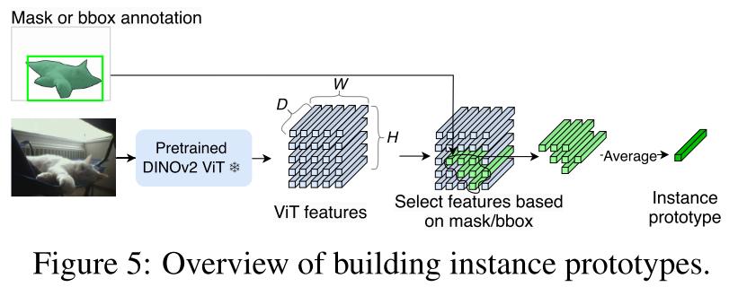
- For each object instance, its prototype is computed as the mean ViT feature from corresponding regions defined by either a segmentation mask or bounding box
- class-representing prototypes are obtained by averaging the cluster centroids of instance-level prototypes for each class
- backgrounds typically share similar visual attributes, such as uniform motion, smooth texture, static color tone, etc
- Because of the lack of visual diversity yet the importance of background semantics, we use masks for a fixed list of background classes, e.g., sky, wall, road, and apply a similar prototype-building procedure