深度学习常用操作 with open 1 2 3 4 5 6 7 8 9 10 11 12 13 14 15 16 17 with open ('filename.txt' , 'r' ) as f: content = f.read(f) with open ('data.txt' , 'w' ) as f: f.write('hello world' ) r: rb: r+: rb+: w: wb: w+: wb+: a: ab: a+: ab+:
计时 python 实现计时器(不同实现方式)
1 2 3 4 5 6 import timetime_start = time.time() time_end = time.time() time_c= time_end - time_start print ('time cost' , time_c, 's' )
log文件夹设置及log使用 1 2 3 4 5 6 7 8 9 10 11 12 13 14 15 16 17 18 19 20 21 22 23 24 25 26 27 28 29 30 31 import datetimeimport jsonsave_dir = os.path.join(args.output_dir, datetime.datetime.now().strftime('%Y-%m-%d-%H-%M' )) log_dir = os.path.join(save_dir, 'log' ) mkdir(log_dir) ckpt_dir = os.path.join(save_dir, 'model' ) mkdir(ckpt_dir) log_file = os.path.join(save_dir, "log.txt" ) train_stats = train(model_without_ddp, device, optimizer, train_loader, epoch, criterion, cam_head, args.n_last_blocks, args.avgpool_patchtokens, mixup_fn) log_stats = {**{f'train_{k} ' : v for k, v in train_stats.items()}, 'epoch' : epoch} if epoch % args.val_freq == 0 or epoch == args.epochs - 1 : test_stats = validate_network(val_loader, model, device, cam_head, args.n_last_blocks, args.avgpool_patchtokens) print ( f"Accuracy at epoch {epoch} of the network on the {len (dataset_val)} test images: {test_stats['acc1' ]:.1 f} %" ) log_stats = {**{k: v for k, v in log_stats.items()}, **{f'test_{k} ' : v for k, v in test_stats.items()}} if utils.is_main_process(): with Path(log_file).open ("a" ) as f: f.write(json.dumps(log_stats) + "\n" ) save_dict = { "epoch" : epoch + 1 , "classifier" : classifier_without_ddp.state_dict(), "model" : model_without_ddp.state_dict(), "optimizer" : optimizer.state_dict(), "scheduler" : scheduler.state_dict(), "best_acc" : best_acc, }
文件/文件夹操作
1 2 3 4 5 6 7 8 import shutilimport errnodef rm (path ): try : shutil.rmtree(path) except OSError as e: if e.errno != errno.ENOENT: raise
1 2 3 4 5 6 7 8 import osimport errnodef mkdir (path ): try : os.makedirs(path) except OSError as e: if e.errno != errno.EEXIST: raise
1 2 3 4 5 6 7 8 9 10 11 12 13 14 15 16 17 import osimport shutilwork_dir = os.getcwd() chip_train_dir = os.path.join(work_dir, "train" + os.sep) if os.path.exists(chip_train_dir): shutil.rmtree(chip_train_dir) if not os.path.isdir(chip_train_dir): os.mkdir(chip_train_dir) def create_output_dir (): if os.path.exists('./output/all' ): shutil.rmtree('./output/all' ) if not os.path.isdir('./output/all' ): os.mkdir('./output/all' ) if os.path.exists(f'./output/{args.method} ' ):
文件夹备份 1 2 3 4 5 6 7 8 9 10 11 12 def backup_codes (root_dir, res_dir, backup_list ): if os.path.exists(res_dir): shutil.rmtree(res_dir) os.makedirs(res_dir) for name in backup_list: shutil.copytree(os.path.join(root_dir, name), os.path.join(res_dir, name)) print ('codes backup at {}' .format (os.path.join(res_dir, name))) backup_dir = os.path.join(cfg.BASIC.SAVE_DIR, 'backup' ) rm(backup_dir) backup_codes(cfg.BASIC.ROOT_DIR, backup_dir, cfg.BASIC.BACKUP_LIST)
文件备份 1 2 3 4 5 6 7 8 9 10 from shutil import copyfiledef backup_codes (root_dir, res_dir, backup_list ): if os.path.exists(res_dir): shutil.rmtree(res_dir) os.makedirs(res_dir) for name in backup_list: copyfile(os.path.join(root_dir, name), os.path.join(res_dir, name)) backup_dir = os.path.join(save_dir, 'backup' ) backup_codes("./" , backup_dir, ['main.py' ])
cfg文件/固定种子 1 2 3 4 5 6 7 8 9 10 11 12 13 14 15 16 17 18 19 20 21 22 23 24 25 26 27 28 29 30 31 32 33 34 class AttrDict (dict ): """ Subclass dict and define getter-setter. This behaves as both dict and obj. """ def __getattr__ (self, key ): return self[key] def __setattr__ (self, key, value ): if key in self.__dict__: self.__dict__[key] = value else : self[key] = value __C = AttrDict() config = __C __C.BASIC = AttrDict() __C.BASIC.TIME = datetime.datetime.now().strftime('%Y-%m-%d-%H-%M' ) __C.BASIC.GPU_ID = [0 ] __C.BASIC.NUM_WORKERS = 0 __C.BASIC.DISP_FREQ = 10 __C.BASIC.SEED = 0 __C.BASIC.SAVE_DIR = '' __C.BASIC.ROOT_DIR = '' __C.BASIC.BACKUP_CODES = True __C.BASIC.BACKUP_LIST = ['lib' , 'tools' , 'tools_cls' ] __C.CUDNN = AttrDict() __C.CUDNN.BENCHMARK = False __C.CUDNN.DETERMINISTIC = True __C.CUDNN.ENABLE = True
1 2 3 4 5 6 7 8 9 10 11 12 13 14 15 16 17 18 19 20 from default import config as cfgimport torchimport randomimport numpy as npdef fix_random_seed (seed ): torch.manual_seed(seed) torch.cuda.manual_seed(seed) torch.cuda.manual_seed_all(seed) np.random.seed(seed) random.seed(seed) def fix_seed_all (cfg ): fix_random_seed(cfg.BASIC.SEED) cudnn.benchmark = cfg.CUDNN.BENCHMARK cudnn.deterministic = cfg.CUDNN.DETERMINISTIC cudnn.enabled = cfg.CUDNN.ENABLE
tensorboard 程序运行时使用writer把数据保存在文件夹中,然后再读取文件夹中的数据
1 2 3 4 5 6 7 8 9 10 11 12 13 14 15 16 17 18 19 from torch.utils.tensorboard import SummaryWriter import datetimesave_dir = os.path.join(args.output_dir, datetime.datetime.now().strftime('%Y-%m-%d-%H-%M' )) log_dir = os.path.join(save_dir, 'log' ) mkdir(log_dir) writer = SummaryWriter(log_dir) writer.add_scalar(tag, scalar_value, global_step=None , walltime=None ) writer.add_scalar('Train_loss' , train_stats['loss' ], global_step=epoch) writer.add_scalar('Learning_rate' , train_stats['lr' ], global_step=epoch) writer.add_scalar('Train Acc_1' , train_stats['acc1' ], global_step=epoch) writer.add_scalar('Acc_1' , test_stats['acc1' ], global_step=epoch) writer.add_scalar('Acc_5' , test_stats['acc5' ], global_step=epoch) writer.add_image(tag, img_tensor, global_step=None , walltime=None , dataformats='CHW' ) writer.add_images(tag, img_tensor, global_step=None , walltime=None , dataformats='NCHW' )
在命令行中
1 2 tensorboard --logdir=./path/to/the/folder --port 8123
1 2 3 4 writer.add_scalar('loss/loss1' , loss1, epoch) writer.add_scalar('loss/loss2' , loss2, epoch) writer.add_scalar('loss/loss3' , loss3, epoch)
tqdm进度条 参考
1 2 3 4 from tqdm import tqdmpbar = tqdm(val_all_dataloader, desc='val' , position=0 ) for batch_idx, (images, labels) in enumerate (pbar): xxxx
tensor变换 torch.stack() 参考
当多个tensor值通过.append()拼接成list格式时,该系列数据是list属性,若需要变为tensor值之后再进行相关操作,可进行如下操作:final_output = torch.stack(output_list)
使用.item()得到张量里的元素值(tensor转为浮点数) 1 2 3 x = torch.randn(1 ) print (x)print (x.item())
Bash脚本 在linux中使用,数字表示变量的顺序,命令行输入时只需要空格分隔跟在后面
1 bash train_val_cub.sh {GPU_ID} ${NET} ${NET_SCALE} ${SIZE}
1 2 3 4 5 6 7 GPU_ID=$1 NET=${2} NET_SCALE=${3} SIZE=${4} export CUDA_VISIBLE_DEVICES=${GPU_ID} python ./tools_cam/train_cam.py --config_file ./configs/CUB/${NET} _tscam_${NET_SCALE} _patch16_${SIZE} .yaml --lr 5e-5 MODEL.CAM_THR 0.1
jupyter notebook 使用 命令行cd到目标文件夹
在jupyter notebook中添加虚拟环境
参考
pycharm 加快debug速度
https://blog.csdn.net/u010087338/article/details/122407903
查看内存使用情况 1 2 3 4 5 6 7 import psutilprint (float (psutil.virtual_memory().total)) print (float (psutil.virtual_memory().used))print (float (psutil.virtual_memory().free))
data Tensor操作 list转tensor 1 2 3 4 x = [] for i in range (length): x.append(xxx) return torch.cat(x, dim=2 )
Tensor变换相关
1 2 cls_label_rep = cls_label.unsqueeze(-1 ).unsqueeze(-1 ).repeat([1 ,1 ,224 ,224 ])
Tensor统计
1 2 3 4 5 6 7 8 9 10 11 12 13 14 15 16 17 18 19 20 21 22 23 pred = torch.tensor([[0.7 ,0 ,0.2 ,0.1 ,0 ],[0 ,0.2 ,0.4 ,0.3 ,0.1 ]]) pred.max (1 , keepdim=True )[1 ] Out: tensor([[0 ],[2 ]]) pred.max (1 , keepdim=True ) Out: torch.return_types.max ( values=tensor([[0.7000 ],[0.4000 ]]), indices=tensor([[0 ],[2 ]])) pred.max (1 , keepdim=False ) Out: torch.return_types.max ( values=tensor([0.7000 , 0.4000 ]), indices=tensor([0 , 2 ])) pred.max (0 , keepdim=False ) Out: torch.return_types.max ( values=tensor([0.7000 , 0.2000 , 0.4000 , 0.3000 , 0.1000 ]), indices=tensor([0 , 1 , 1 , 1 , 1 ]))
数组索引 使用tuple作为索引
array[tuple]
unnormalize image 1 2 3 4 5 6 7 def unnormalize_images (images ): mean = [0.485 , 0.456 , 0.406 ] std = [0.229 , 0.224 , 0.225 ] mean = torch.reshape(torch.tensor(mean), (1 , 3 , 1 , 1 )) std = torch.reshape(torch.tensor(std), (1 , 3 , 1 , 1 )) unnormalized_images = images.clone().detach().cpu() * std + mean return unnormalized_images
PIL 读取、保存、显示 1 2 3 4 5 6 from PIL import ImageDraw, Imageimage = Image.open (path).convert('RGB' ) draw = ImageDraw.Draw(image) draw.rectangle([sample.xmin, sample.ymin, sample.xmax, sample.ymax], outline=(255 , 0 , 0 )) image.show()
ndarray形式的CAMs和图像叠加显示 需要注意,要把bgr顺序转为rgb,否则heatmap变coldmap
1 2 3 4 5 6 7 import cv2from PIL import Imageheatmap = cv2.applyColorMap(cv2.resize(CAMs, (224 , 224 )), cv2.COLORMAP_JET) heatmap = cv2.cvtColor(heatmap, cv2.COLOR_BGR2RGB) result = heatmap * 0.3 + image * 0.5 Image.fromarray(np.uint8(heatmap)).save(heatmap_name) Image.fromarray(np.uint8(result)).save(result_name)
使用PIL进行图像的padding(加灰条) 1 2 3 4 5 6 7 8 9 image = Image.open (path).convert('RGB' ) w, h = image.size background = Image.new('RGB' , size=(max (w, h), max (w, h)), color=(235 , 235 , 235 )) length = int (abs (w - h) // 2 ) box = (length, 0 ) if w < h else (0 , length) background.paste(image, box) background.show() image = background image = self.transform(image)
matplotlib 使用plt.imsave将灰度图保存为伪彩色图 1 2 3 4 plt.imshow(attentions[j]) plt.colorbar() plt.imsave(fname=pltname, arr=eigvec, cmap='cividis' )
1 2 3 4 5 6 7 8 9 10 11 12 13 14 15 16 17 18 19 20 import matplotlib.pyplot as pltattentions = model.get_last_selfattention(img.to(device)) nh = attentions.shape[1 ] attentions = attentions[0 , :, 0 , 1 :].reshape(nh, -1 ) attentions = attentions.reshape(nh, w_featmap, h_featmap) attentions = nn.functional.interpolate(attentions.unsqueeze(0 ), scale_factor=args.patch_size, mode="nearest" )[0 ].cpu().numpy() for j in range (nh): fname = os.path.join(args.output_dir, "attn-head" + str (j) + ".png" ) plt.imshow(attentions[j]) plt.colorbar() plt.imsave(fname=fname, arr=attentions[j], format ='png' ) print (f"{fname} saved." )
TokenCut中的可视化
注意cmap指color map,也就是选择伪彩色图的类型
1 2 3 4 5 6 def visualize_eigvec (eigvec, folder, im_name, dim, scales, save=True ): eigvec = scipy.ndimage.zoom(eigvec, scales, order=0 , mode='nearest' ) if save: pltname= f"{folder} /{im_name} _ours_att.jpg" plt.imsave(fname=pltname, arr=eigvec, cmap='cividis' )
OpenCV cv的输入数据类型不能是tensor,需要转换为ndarray
图像的通道顺序 1 2 3 4 5 6 7 8 9 10 11 import cv2img = cv2.imread(img_path) b, g, r = cv2.split(img) img1 = cv2.merge([r, g, b]) img3 = cv2.cvtColor(img, cv2.COLOR_BGR2RGB) cv2.imwrite(filename,img)
cv2.resize() 参考
在使用opencv -python中的cv2.resize()函数进行图片缩放时,输入参数中的dsize,即输出图片的大小,顺序应为(w, h),和cv2.imread()读入图片的顺序相反,cv2.imread()读入图片的通道顺序为(h, w, c)。
1 2 3 4 5 6 7 8 9 10 11 12 13 14 15 16 cam_map_ = cam_map_.detach().cpu().numpy().transpose(1 , 2 , 0 ) cam_map_ = resize_cam(cam_map_, size=(crop_size, crop_size)) def resize_cam (cam, size=(224 , 224 ): cam = cv2.resize(cam, (size[0 ], size[1 ])) cam_min, cam_max = cam.min (), cam.max () cam = (cam - cam_min) / (cam_max - cam_min) return cam seed_patch = np.zeros(196 ) seed_patch[seed] = 1 seed_patch = seed_patch.reshape(14 , 14 ) seed_patch = cv2.resize(seed_patch, (224 , 224 ), interpolation=cv2.INTER_NEAREST)
cv2.imshow() 1 2 cv2.imshow("Image-New" , thr_gray_heatmap) cv2.waitKey(0 )
横向纵向排列图片 1 2 htitch= np.hstack((img1, img3,img4)) vtitch = np.vstack((img1, img3))
图像与运算 1 final_out = cv2.bitwise_and(close_out, reliable_back_label)
开运算和闭运算 参考
保存cam图像(原本是0-1值的) 1 2 3 4 5 6 7 8 9 10 11 12 13 save_dir = 'test_visualize' save_path_img = 'test_visualize/ori-img.jpg' save_path_cam = 'test_visualize/cam.jpg' mkdir(save_dir) cam_b = (cam_b * 255. ).astype(np.uint8) cv2.imwrite(save_path_img, image[b]) cv2.imwrite(save_path_cam, cam_b) save_path_img = 'ori-img.jpg' save_path_cam = 'cam.jpg' rgb_img = cv2.imread(save_path_img, 1 ) cam = cv2.imread(save_path_cam, 0 )
设置指定颜色 1 2 3 4 5 6 cls_loss_label = np.ones((224 , 224 , 3 )) cls_loss_label[background_label == 0 ] = [77 , 34 , 1 ] cls_loss_label[obj_label == 255 ] = [55 , 232 , 253 ] cls_loss_label = np.where((cls_loss_label == [1 , 1 , 1 ]).all (axis=-1 )[..., None ], [0 , 0 , 255 ], cls_loss_label) cv2.imwrite('./draw_for_paper/cls_loss_label_ori.jpg' , cls_loss_label)
去除小连通域 https://blog.csdn.net/ayinaaaa/article/details/121499851
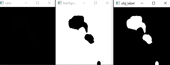
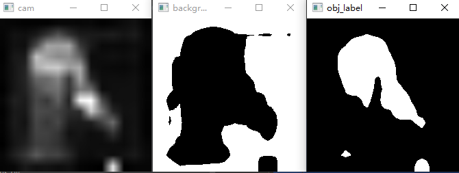
利用cv2.threshold()获取高低置信度区域 1 2 3 4 5 6 7 8 9 10 11 cv2.imshow("cam" , cam) back_thr = cam_thr_back * np.max (cam) _, background_label = cv2.threshold(cam, int (back_thr), 255 , cv2.THRESH_BINARY_INV) cv2.imshow("background_label" , background_label) obj_thr = cam_thr_obj * np.max (cam) _, obj_label = cv2.threshold(cam, int (obj_thr), 255 , cv2.THRESH_BINARY) cv2.imshow("obj_label" , obj_label)
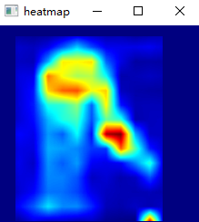
利用cv2.applyColorMap()彩色可视化二维灰度图像 需要注意2维ndarray元素数据类型必须转换成np.uint8类型
1 2 3 4 5 6 7 8 9 I = np.zeros_like(cam) x1, y1, x2, y2 = es_box I[y1:y2, x1:x2] = 1 cam = cam * I cam = cam.astype(np.uint8) heatmap = cv2.applyColorMap(cam, cv2.COLORMAP_JET) cv2.imshow("heatmap" , heatmap)
cv2.threshold() + cv2.findContours()获取外接矩形 cv2.threshold()和findContours()都不会修改输入图像
画图的函数,一般最后两个参数分别是color和线粗,且是在输入图像上原地操作,所以可以使用img.copy()
1 2 cv2.drawContours(thr_gray_heatmap, contours, -1 , (255 , 0 , 0 ), 3 ) cv2.rectangle(thr_gray_heatmap, (x, y), (x+w, y+h), (255 , 0 , 0 ), 2 )
img.copy()
参考 参考,轮廓检测
1 2 3 4 5 6 7 8 9 10 11 12 13 14 15 16 17 18 19 20 21 22 23 24 25 26 27 28 29 30 31 32 33 34 35 36 37 38 39 def get_bboxes (cam, cam_thr=0.2 ): """ cam: single image with shape (h, w, 1) thr_val: float value (0~1) return estimated bounding box """ cam = (cam * 255. ).astype(np.uint8) map_thr = cam_thr * np.max (cam) cv2.imshow("Image-Old" , cam) _, thr_gray_heatmap = cv2.threshold(cam, int (map_thr), 255 , cv2.THRESH_TOZERO) cv2.imshow("Image-New" , thr_gray_heatmap) contours, _ = cv2.findContours(thr_gray_heatmap, cv2.RETR_TREE, cv2.CHAIN_APPROX_SIMPLE) cv2.drawContours(thr_gray_heatmap, contours, -1 , (255 , 0 , 0 ), 3 ) cv2.imshow("drawContours" , thr_gray_heatmap) if len (contours) != 0 : c = max (contours, key=cv2.contourArea) x, y, w, h = cv2.boundingRect(c) estimated_bbox = [x, y, x + w, y + h] cv2.rectangle(thr_gray_heatmap, (x, y), (x+w, y+h), (255 , 0 , 0 ), 2 ) cv2.imshow("rectangle" , thr_gray_heatmap) cv2.waitKey(0 ) else : estimated_bbox = [0 , 0 , 1 , 1 ] return estimated_bbox
存疑
findContours的输入要求是二值图像,但这里传入灰度图也正常运行了
cv2.drawContours(thr_gray_heatmap, contours, -1, (255, 0, 0), 3)用imshow查看结果,在原本的灰度图上画了白色的线,没有画出红色的线
cv2.drawContours(cam, contours, -1, (255, 0, 0), 3)运行不会产生线
画超像素边界 1 2 3 4 5 if (cnt_i == 20 ): spixel_bd_image = mark_boundaries(image, seg_map, color=(0 , 255 , 255 )) cv2.imwrite('./draw_for_paper/image.jpg' , image) spixel_bd_image = spixel_bd_image + image cv2.imwrite('./draw_for_paper/spixel_bd_image.jpg' , spixel_bd_image)
5种裁剪方式 参考
随机裁剪 transforms.RandomCrop(size,padding=None,pad_if_need=False,fill=0,padding_mode=’constant’)
size:要么是(h,w),若是一个int,就是(size,size)
可以使用padding进行填充,值由fill决定,可以是(R,G,B)
中心裁剪 transforms.CenterCrop(size)
从中心裁剪出(size, size)的区域
随机长宽比裁剪 transforms.RandomResizedCrop(size,scale=(0.08,1.0),ratio=(0.75,1.33),interpolation=2)
将给定图像随机裁剪为不同的大小和宽高比,然后缩放所裁剪得到的图像为制定的大小
即先随机采集,然后对裁剪得到的图像缩放为同一大小,随机裁剪后的大小: (size, size)
上下左右中心裁剪 transforms.FiveCrop(size)
对图片进行上下左右以及中心的裁剪,获得五张图片,返回一个4D的tensor
上下左右中心裁剪后翻转 transforms.TenCrop(size,vertical_flip=False)
对图片进行上下左右以及中心裁剪,然后全部翻转(水平或者垂直,总共获得十张图片)
示例1 参考
transforms.RandomResizedCrop(224)
将给定图像随机裁剪为不同的大小和宽高比,然后缩放所裁剪得到的图像为制定的大小
即先随机采集,然后对裁剪得到的图像缩放为同一大小,随机裁剪后的大小: (224, 224)
transforms.RandomHorizontalFlip()
以给定的概率随机水平旋转给定的PIL的图像,默认为0.5
1 2 3 4 5 import torchvision.transforms as transformstransforms.Compose([transforms.RandomResizedCrop(224 ), transforms.RandomHorizontalFlip(), transforms.ToTensor(), transforms.Normalize([0.485 , 0.456 , 0.406 ], [0.229 , 0.224 , 0.225 ])])
示例2 (TS-CAM)
transforms.Resize(x), 对象必须是PIL Image,不能是io.imread或cv2.imread读取的图片,这两种得到的是ndarray
将图片短边缩放至x,长宽比保持不变
transforms.Resize([h, w])
指定长宽
1 2 3 4 5 6 7 8 9 10 11 12 13 14 15 16 train_transform = transforms.Compose([ transforms.Resize((cfg.DATA.RESIZE_SIZE, cfg.DATA.RESIZE_SIZE)), transforms.RandomCrop((cfg.DATA.CROP_SIZE, cfg.DATA.CROP_SIZE)), transforms.RandomHorizontalFlip(), transforms.ToTensor(), transforms.Normalize(cfg.DATA.IMAGE_MEAN, cfg.DATA.IMAGE_STD) ]) test_transform = transforms.Compose([ transforms.Resize((cfg.DATA.CROP_SIZE, cfg.DATA.CROP_SIZE)), transforms.ToTensor(), transforms.Normalize(cfg.DATA.IMAGE_MEAN, cfg.DATA.IMAGE_STD) ])
示例3 (TokenCut) 1 2 3 4 5 6 7 8 9 10 11 12 13 14 resize_im = args.input_size > 32 if is_train: transform = transforms.Compose([ transforms.RandomResizedCrop(args.input_size), transforms.RandomHorizontalFlip(), transforms.ToTensor(), transforms.Normalize((0.485 , 0.456 , 0.406 ), (0.229 , 0.224 , 0.225 )), ]) if not resize_im: transform.transforms[0 ] = transforms.RandomCrop( args.input_size, padding=4 ) return transform
model 导入预训练权重的部分参数 导入预训练权重的部分参数
PyTorch 多 GPU 训练保存模型权重 key 多了 ‘module.‘
1 2 3 4 5 6 7 8 9 10 11 12 13 14 15 16 17 18 19 20 21 22 23 24 25 26 27 model = create_deit_model( cfg.MODEL.ARCH, pretrained=False , num_classes=cfg.DATA.NUM_CLASSES, drop_rate=args.drop, drop_path_rate=args.drop_path, drop_block_rate=None , ) checkpoint_path = './pretrained_weight/model_epoch60_small.pth' tscam_model = torch.load(checkpoint_path)['state_dict' ] weights_dict = {} for k, v in tscam_model.items(): new_k = k.replace('module.' , '' ) if 'module' in k else k weights_dict[new_k] = v tscam_model = weights_dict model_dict = model.state_dict() state_dict = {k: v for k, v in tscam_model.items() if k in model_dict.keys()} model_dict.update(state_dict) model.load_state_dict(model_dict)
1 2 3 4 5 6 7 8 9 10 11 12 13 linear_classifier = LinearClassifier(embed_dim, num_labels=args.num_labels) linear_classifier = linear_classifier.cuda() linear_ckpt_path = './pretrained_weight/model_best.pth' linear_model = torch.load(linear_ckpt_path) weights_dict = {} for k, v in linear_model.items(): new_k = k.replace('module.' , '' ) if 'module' in k else k weights_dict[new_k] = v linear_model = weights_dict linear_classifier_dict = linear_classifier.state_dict() state_dict = {k: v for k, v in linear_model['classifier' ].items() if k in linear_classifier_dict.keys()} linear_classifier_dict.update(state_dict) linear_classifier.load_state_dict(linear_classifier_dict)
nn.Parameter() 1 self.v = torch.nn.Parameter(torch.FloatTensor(hidden_size))
将一个固定不可训练的tensor转换成可以训练的类型parameter,并将这个parameter绑定到这个module里面(net.parameter()中就有这个绑定的parameter),所以经过类型转换这个self.v变成了模型的一部分,成为了模型中根据训练可以学习改动的参数了。
nn.Module中的self.register_buffer() 参考
F.pad 参考
1 2 3 4 5 6 7 8 9 10 11 12 13 14 torch.nn.functional.pad(input , pad, mode,value ) Args: """ input:四维或者五维的tensor Variabe pad:不同Tensor的填充方式 1.四维Tensor:传入四元素tuple(pad_l, pad_r, pad_t, pad_b), 指的是(左填充,右填充,上填充,下填充),其数值代表填充次数 2.六维Tensor:传入六元素tuple(pleft, pright, ptop, pbottom, pfront, pback), 指的是(左填充,右填充,上填充,下填充,前填充,后填充),其数值代表填充次数 mode: ’constant‘, ‘reflect’ or ‘replicate’三种模式,指的是常量,反射,复制三种模式 复制模式就是把最边上值的复制n次 value:填充的数值,在"contant"模式下默认填充0,mode="reflect" or "replicate"时没有 value参数 """
F.conv2d 参考
nn.Conved是2D卷积层,而F.conv2d是2D卷积操作
1 2 3 4 5 6 7 8 9 10 11 12 13 14 15 16 17 18 import torchfrom torch.nn import functional as F """手动定义卷积核(weight)和偏置""" w = torch.rand(16 , 3 , 5 , 5 ) b = torch.rand(16 ) """定义输入样本""" x = torch.randn(1 , 3 , 28 , 28 ) """2D卷积得到输出""" out = F.conv2d(x, w, b, stride=1 , padding=1 ) print (out.shape) out = F.conv2d(x, w, b, stride=2 , padding=2 ) print (out.shape)out = F.conv2d(x, w) print (out.shape)
空洞卷积
1 2 mu1 = F.conv2d(img1, window , padding=padd, dilation=dilation, groups=channel)
F.interpolate——数组采样操作 参考
train 冻结部分参数进行训练 参考1
参考2
1 2 3 4 5 6 7 8 9 10 11 12 13 14 15 16 17 model_dict = model.state_dict() dict_name = list (model_dict) for i, p in enumerate (dict_name): print (i, p) for i, (name, p) in enumerate (model.named_parameters()): if i < 150 : print (name) p.requires_grad = False for i, (name, p) in enumerate (model.named_parameters()): print (p.requires_grad) for param in model.parameters(): param.requires_grad = True for i, (name, p) in enumerate (model.named_parameters()): print (p.requires_grad)
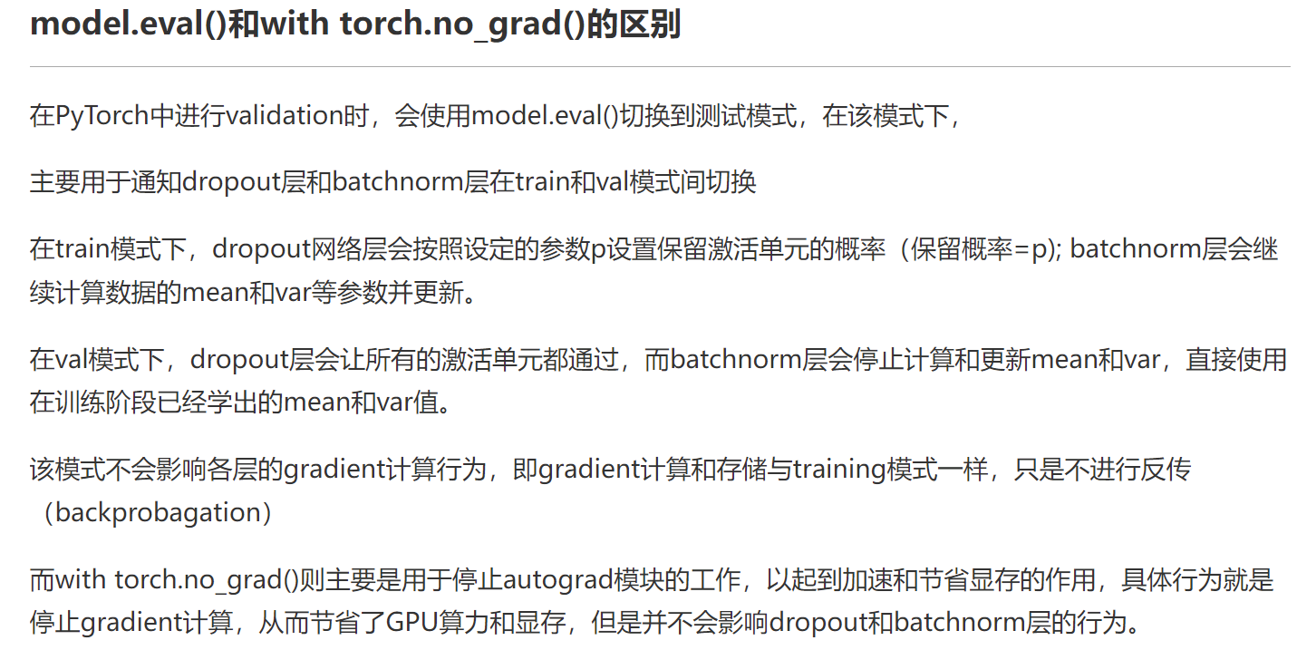
optimizer eval .eval的作用,为什么在eval阶段使用with torch.no_grad()
loss function Cross entropy 参考
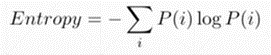
熵:描述了一个分布
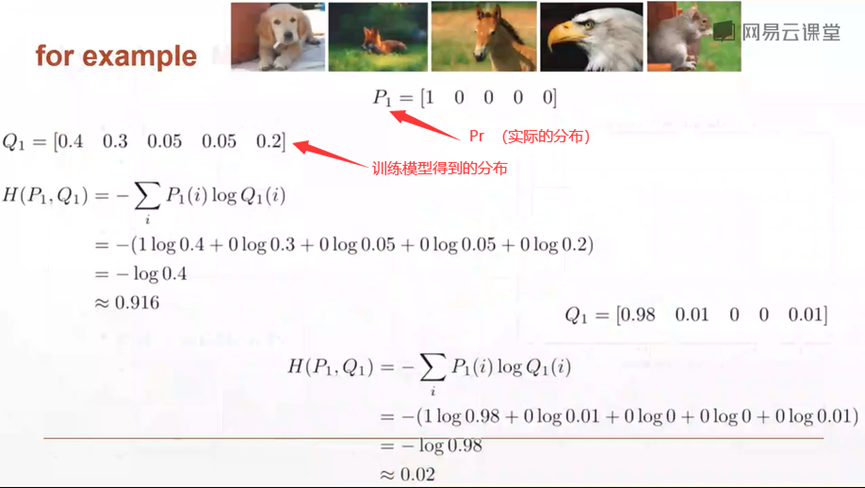
交叉熵:$H(p,q)=-\sum p(x)logq(x)$
又可以写成: $H(p,q)=H(p)+D_{KL}(p|q)$
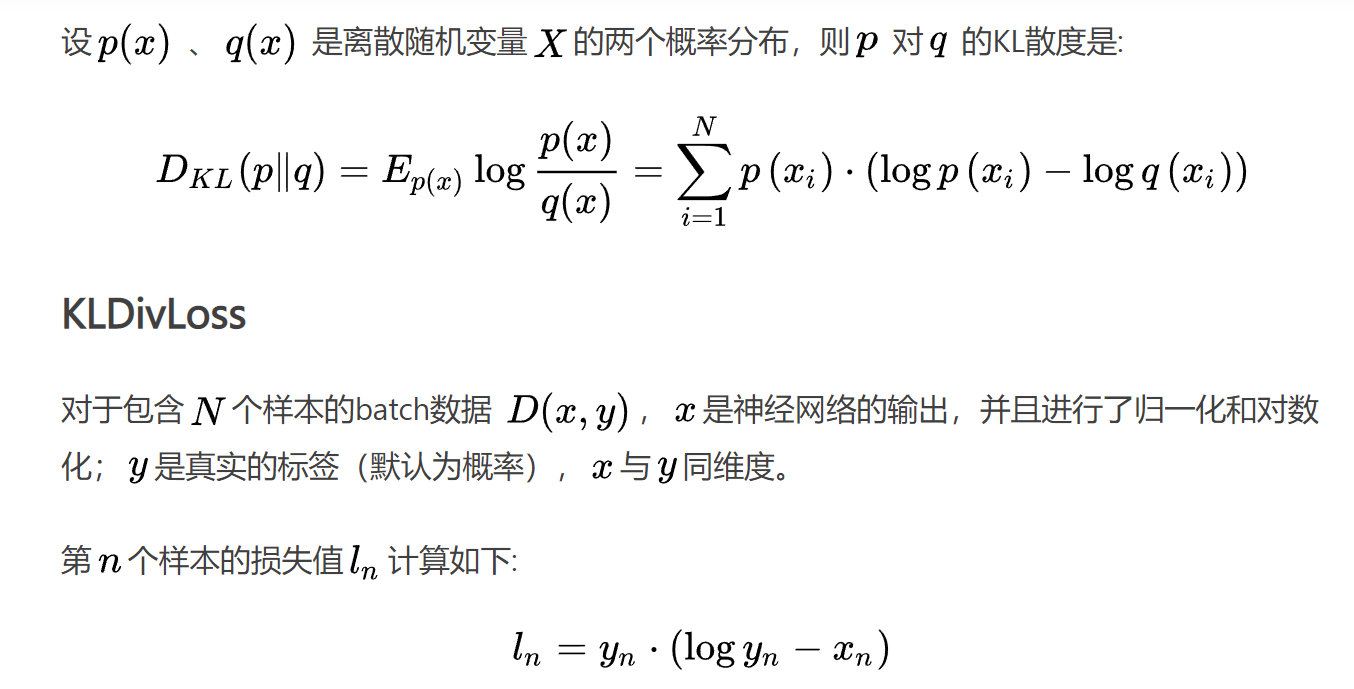
其中$D_{KL}$指KL Divergence,描述两个分布的重合程度,当p和q两个分布相似时,散度接近于0
在使用Cross entropy作为损失函数时,可以将q认为是训练的模型得到分布,p是实际模型的分布(也就是ground truth)
cross_entropy=softmax+log+nll_loss
1 2 criteon = nn.CrossEntropyLoss() loss = criteon(logits, target)
需要注意的是Pytorch中的F.cross_entropy或nn.CrossEntropyLoss()必须传入的是logits(未经softmax处理的),因为这里的F.cross_entropy已经包含了softmax,也就是说F.cross_entropy=softmax+log+nll_loss
参考
使用softmax对logits进行计算,得到每张图片的概率分布,值为0-1,概率之和为1
对softmax的结果取自然对数,因为softmax后的数值为0-1,所以取了ln后值域为负无穷到0
然后进行NLL Loss计算,NLL Loss的结果就是将上一步骤的值去掉负号求均值
CrossEntropyLoss就是把上述三个步骤softmax+log+nll_loss合并为一步
二元交叉熵 https://blog.csdn.net/qq_36158230/article/details/124071087
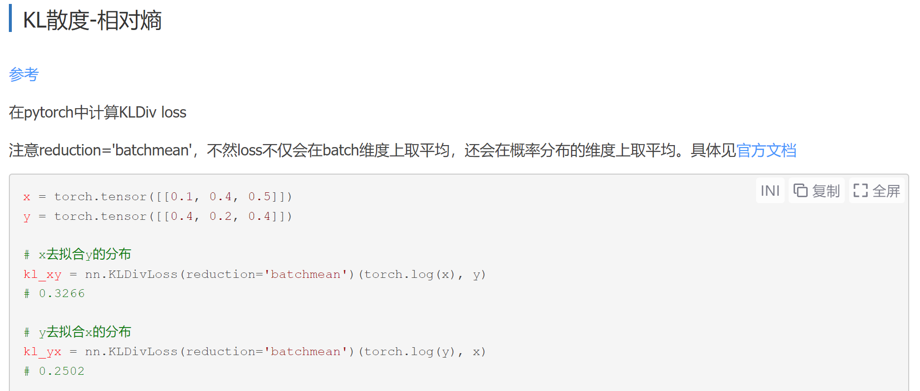
KLDivLoss KLDivLoss
pytorch
1 2 3 4 5 hard_criterion = nn.CrossEntropyLoss() soft_criterion = nn.KLDivLoss(reduction="batchmean" ) hard_loss = hard_criterion(output, target) KD_loss = soft_criterion(torch.log(F.softmax(output/temp, dim=1 )), F.softmax(linear_output/temp, dim=1 ))
常见问题 参数不更新的常见原因:
参考
loss出现NaN
1.如果在迭代的100轮以内,出现NaN,一般情况下的原因是因为你的学习率过高,需要降低学习率。可以不断降低学习率直至不出现NaN为止,一般来说低于现有学习率1-10倍即可。
2.如果当前的网络是类似于RNN的循环神经网络的话,出现NaN可能是因为梯度爆炸的原因,一个有效的方式是增加“gradient clipping”(梯度截断来解决)
3.可能用0作为了除数;
4.可能0或者负数作为自然对数
5.需要计算loss的数组越界(尤其是自己,自定义了一个新的网络,可能出现这种情况)
6.在某些涉及指数计算,可能最后算得值为INF(无穷)(比如不做其他处理的softmax中分子分母需要计算exp(x),值过大,最后可能为INF/INF,得到NaN,此时你要确认你使用的softmax中在计算exp(x)做了相关处理(比如减去最大值等等))